TOWARDS ENHANCING TIME SERIES CONTRASTIVE LEARNING- A DYNAMIC BAD PAIR MINING APPROACH

Introduction

Contrastive learning 이란?

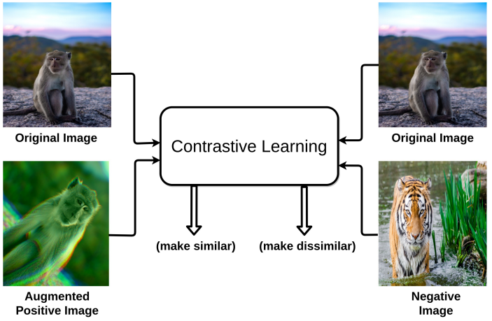
• The key concept of time series contrastive learning is to capture the meaningful underlying information shared between views (usually generated by random data augmentation), such that the learned representations are discriminative among time series.
• To accomplish this objective, existing contrastive methods comply with an assumption that the augmented views from the same instance (i.e., positive pair) share meaningful semantic information

Contrastive learning의 문제점

• It was discovered that the effectiveness of the contrastive learning models will indeed suffer when two views generated from the same image actually do not share meaningful information (e.g., an unrelated cat-dog pair cropped from the same image
• In other words, not all positive pairs are beneficial to contrastive learning.

Noisy Positive pairs

• This results in noisy contrasting views, where the shared information between views is predominantly noise.
• As a result, a noisy alignment occurs, in which the model simply learns the pattern of noise rather than the true signal.

Faulty positive pairs

• Due to the sensitivity of time series, data augmentation may inadvertently impair sophisticated temporal patterns contained in the original signal and thus produce faulty views.
• Consequently, the augmented view is no longer has the same semantic meaning as the original ECG, leading to a faulty alignment where the model learns to align non-representative patterns shared between views.

An intuitive solution is to suppress bad positive pairs during contrastive training, however, directly identifying bad positive pairs in real-world datasets is challenging for two reasons.

• First, for noisy positive pairs, it is often infeasible to measure the noise level given a signal from a real-world dataset.
• Second, for faulty positive pairs, one will not be able to identify if the semantic meaning of augmented views are changed without the ground truth.

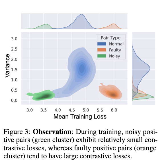
We find noisy positive pairs exhibit relatively small losses throughout the training process. In contrast, faulty positive pairs are often associated with large losses during training.

Dynamic bad pair mining (DBPM) algorithm.

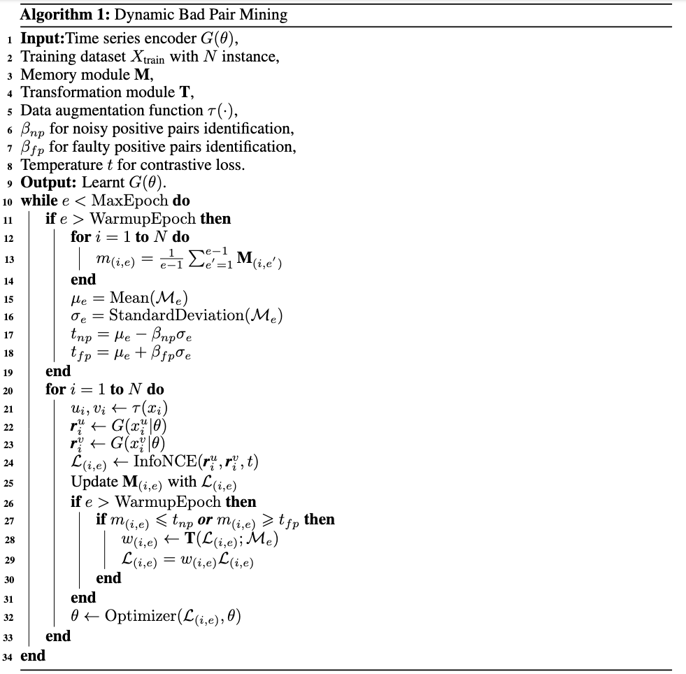
• we design a dynamic bad pair mining (DBPM) algorithm.
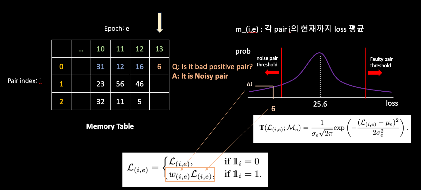
• The proposed DBPM algorithm addresses the bad positive pair problem with a simple concept: identify and suppress.
• Specifically, DBPM aims for reliable bad positive pair mining and down-weighting in the contrastive training.
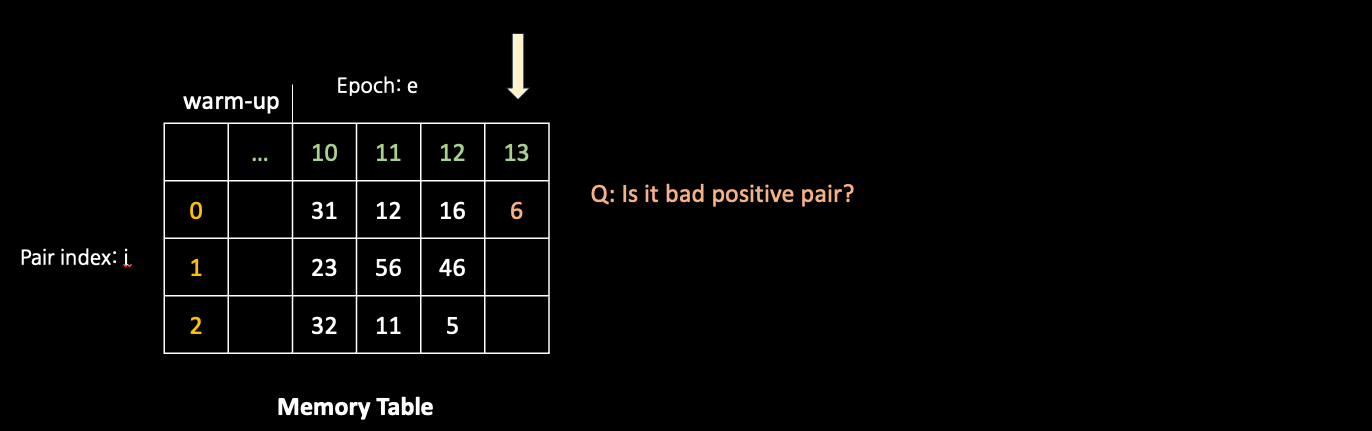
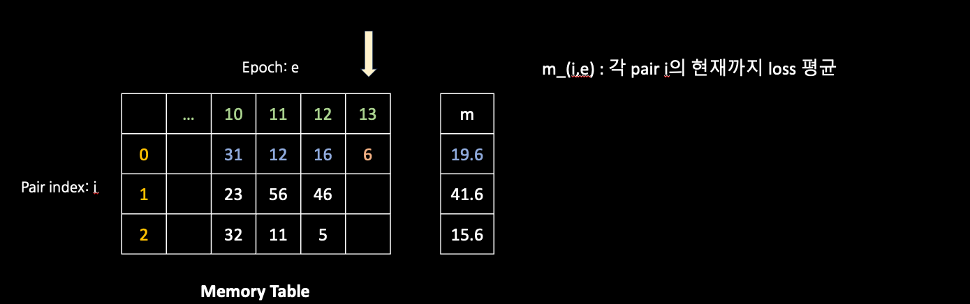
• To this end, DBPM first utilizes a memory module to track the training behavior of each pair along training process.

Contribution

First, to the best of our knowledge, this is the first study to investigate the bad positive pair problem exists in time series contrastive learning. Our study contributes to a deeper understanding of an important issue that has not been thoroughly explored. Second, we propose DBPM, a simple yet effective algorithm designed as a lightweight plug-in that dynamically deals with potential bad positive pairs along the contrastive learning process, thereby improving the quality of learned time series representations. Third, extensive experiments over four real-world large-scale time series datasets demonstrate the efficacy of DBPM in enhancing the performance of existing state-of-the-art methods.

Related works

Our DBPM differs from image-based solutions in following aspects.

• First, DBPM is designed for time series contrastive learning, in which not only faulty positive pairs arise, but also noisy positive pairs exist. The particular challenge of addressing two different types of bad positive pairs is unique to time series data and distinguishes them from image data.
• Furthermore, DBPM identifies bad positive pairs based on their historical training behaviors in a dynamic manner, which allows more reliable identification of potential bad positive pairs.

Methods

Problem definition

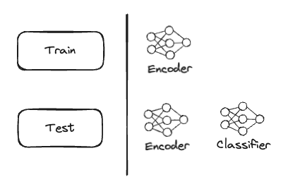
• Linear probing을 통한 contrastive learning 성능 확인

ANALYSIS: TIME SERIES CONTRASTIVE LEARNING

Symbols

• $x_i$: A training time series instance in the dataset.
• ${\mathbb{R}}^{C\times K}$: The real coordinate space of the time series data, with $C$ channels and $K$ time points.
• ${\mathcal{X}}_{\text{train}}$: The training set containing all time series instances.
• $N$: The total number of instances in the training set.
• $\tau (\cdot )$: A random data augmentation function applied to the time series data.
• $(u_i,v_i)$: A pair of different views generated from the original data $x_i$ by the augmentation function $\tau$, representing a positive pair.
• $G(\cdot |\theta )$: The time series encoder function parameterized by $\theta$.
• $r_i^u,r_i^v$: Representations of the views $u_i$ and $v_i$ in the representation space, as encoded by $G$.
• $\mathcal{L}(u_i,v_i)$: The contrastive loss for a pair of views $u_i$ and $v_i$.
• $s(r^u,r^v)$: A score function, specifically the dot product between normalized representations $r^u$ and $r^v$.
• $t$: A temperature parameter that scales the contrastive loss.
• $z_i$: The true signal in the input data that contains desired features for the encoder to learn.
• ${\xi }_i$: Spurious dense noise present in the input data.
• $D_z,D_{\xi }$: Distributions representing the true signal and the noise, respectively.
• $\arg {\max }_{\theta }$: An operator that finds the values of $\theta$ that maximize the given function.
• $I(\cdot ;\cdot )$: Mutual information between the representations of two views.
• $D_{\text{unknown}}$: A distribution representing an unknown or faulty signal not aligned with the true signal $D_z$.
• $\frac{\partial \mathcal{L}}{\partial r_i^u}$: The partial derivative of the contrastive loss with respect to the representation $r_i^u$.

Preliminaries.

Consider a training time series $x_i\in {\mathbb{R}}^{C\times K}$ in a training set ${\mathcal{X}}_{\text{train}}$ with $N$ instance, the time series contrastive learning framework first applies a random data augmentation function $\tau (\cdot )$ to generate two different views from original data $(u_i,v_i)=\tau (x_i)$ (i.e., positive pair). These two views are then projected to representation space by the time series encoder $(r_i^u,r_i^v)=(G(u_i|\theta ),G(v_i|\theta ))$. The time series encoder is learned to maximize the agreement between positive pair $(u_i,v_i)$ by minimizing the contrastive loss (i.e., InfoNCE): The contrastive loss $\mathcal{L}(u_i,v_i)$ is defined as:

$$\mathcal{L}(u_i,v_i)=-\log \frac{\exp (s(r_i^u,r_i^v)/t)}{\exp (s(r_i^u,r_i^v)/t)+{\sum }_{j=1}^N\exp (s(r_i^u,r_i^j)/t)},$$

where $s(r^u,r^v)=(r^u\cdot r^v)/\Vert r^u\Vert \Vert r^v\Vert$ is a score function that calculates the dot product between ${\ell }_2$ normalized representation $r^u$ and $r^v$. $(r_i^u,r_i^j)$ denotes representations from different time series (i.e., negative pairs). $t$ is a temperature parameter.

Noisy Alignment

Let us consider the noisy positive pair problem. According to [Wen & Li, 2021], each input data can be represented in the form of $x_i=z_i+{\xi }_i$, where $z_i\sim D_z$ denotes the true signal that contains the desired features we want the encoder $G(\theta )$ to learn, and ${\xi }_i\sim D_{\xi }$ is the spurious dense noise. We hypothesize that the noisy positive pair problem is likely to occur on $x_i$ when ${\xi }_i>>z_i$, because noisy raw signals will produce noisy views after data augmentation. Formally, we define $(u_i,v_i)$ as a noisy positive pair when ${\xi }_i^u>>z_i^u$ and ${\xi }_i^v>>z_i^v$. Further, we know that minimizing the contrastive loss is equivalent to maximize the mutual information between the representations of two views [Tian et al., 2020]. Therefore, when noisy positive pairs present, $\arg {\max }_{\theta }I(G(u_i|\theta );G(v_i|\theta ))$ is approximate to $\arg {\max }_{\theta }I(G({\xi }_i^u|\theta );G({\xi }_i^v|\theta ))$. This results in noisy alignment, where the model predominantly learning patterns from noise.

Faulty Alignment

Now, we consider the faulty positive pair problem. In view of the sensitivity of time series, it is possible that random data augmentations (e.g., permutation, cropping [Um et al., 2017]) alter or impair the semantic information contained in the original time series, thus producing faulty views. Formally, we define $(u_i,v_i)$ as a faulty positive pair when $\tau (x_i)\sim D_{\text{unknown}}$, where $D_{\text{unknown}}\ne D_z$. Take partial derivatives of $\mathcal{L}(u_i,v_i)$ w.r.t. $r_i^u$ (full derivation in Appendix A.4), we have

$$-\frac{\partial \mathcal{L}}{\partial r_i^u}=\frac{1}{t}\left(r_i^v-\sum _{j=0}^N\frac{r_i^j\exp (s(r_i^u,r_i^j)/t)}{{\sum }_{j=0}^N\exp (s(r_i^u,r_i^j)/t)}\right),$$

Eq.2 reveals that the representation of augmented view $u_i$ depends on the representation of augmented view $v_i$, and vice versa. This is how alignment of positive pairs happens in contrastive learning: the two augmented views $u_i$ and $v_i$ provide a supervision signal to each other. For example, when $v_i$ is a faulty view (i.e., $z_i^v\sim D_z$, $z_i^v\sim D_{\text{unknown}}$), $r_i^v$ provides a false supervision signal to $G(\theta )$ to learn $r_i^u$. In such a case, $\arg {\max }_{\theta }I(r_i^u;r_i^v)$ is approximate to $\arg {\max }_{\theta }I(G(z_i^u|\theta );G(z_i^v|\theta ))$, where $G(\theta )$ extracts faulty or irrelevant information shared between $u_i$ and $v_i$, leading to a faulty alignment. This analysis can also be applied to situations where $u_i$ is a faulty view, or where both $u_i$ and $v_i$ are faulty views. Moreover, we hypothesize that representations from faulty positive pairs often exhibit low similarity (i.e., $s(r_i^u,r_i^v)\downarrow$), as their temporal patterns are different. This means the encoder will place larger gradient on faulty positive pairs, which exacerbates the faulty alignment.

Empirical evidence

• We pre-define three types of positive pair in our simulated dataset: normal positive pair, noisy positive pair, and faulty positive pair.
• In order to simulate noisy positive pairs, we assume that the noise level of a signal depends on its Signal-to-Noise Ratio (SNR). By adjusting the SNR, we can generate time series with varying levels of noise, from clean (i.e., SNR>1) to extremely noisy (i.e., SNR<1).
• To simulate faulty positive pairs, we randomly select a portion of data and alter their temporal features to produce faulty views.
• We find that noisy positive pairs exhibit a relatively small loss and variance throughout the training process (the green cluster)
• In contrast, faulty positive pairs are often associated with large contrastive loss and small variance during training (the orange cluster), which implies that the faulty positive pair is difficult to align.

Dynamic Bad Pair Mining

Graphical Description

Code

 
#* calculate weighted average training loss for each instance 
epoch_weight = [(1+i)/self.config['trainer']['max_epochs'] for i in range(epoch)]
instance_mean = {k: np.mean(np.array(v)*epoch_weight) for k, v in sorted(memory_module.items(), key=lambda item: item[1])}
 
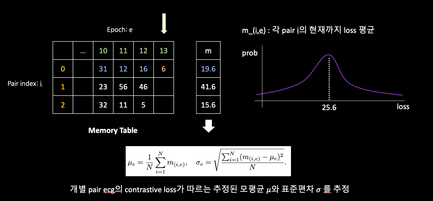
mu = np.mean(list(instance_mean.values()))
sd = np.std(list(instance_mean.values()))
 
#* global statistic
gaussian_norm = norm(mu, sd)
 
#* thresholds for noisy positive pairs and faulty positive pairs
np_bound = mu-self.config['correction']['cut_np']*sd
fp_bound = mu+self.config['correction']['cut_fp']*sd
 
#* identify potential bad positive pairs
np_index = [k for k in instance_mean.keys() if instance_mean[k]<=np_bound]
fp_index = [k for k in instance_mean.keys() if instance_mean[k]>=fp_bound]
 

z1 = self.head(self.encoder(x1))
z2 = self.head(self.encoder(x2))
 
pos_loss = loss_ntxent([z1, z2], self.device)
 
#* update the memory module
for i in range(len(index)):
memory_module[index[i].cpu().item()].append(pos_loss[i].cpu().item())
 
#* DBPM re-weighting process
if epoch >= self.config['trainer']['warm_epochs']:
	l = pos_loss.detach().cpu()
	w = gaussian_norm.pdf(l)
	for i in range(len(index)):
		_id = index[i].cpu().item()
		if _id in np_index:
			#* penalize potential np
			pos_loss[i] *= w[i]
		elif _id in fp_index:
			#* penalize potential fp  
			pos_loss[i] *= w[i]
 

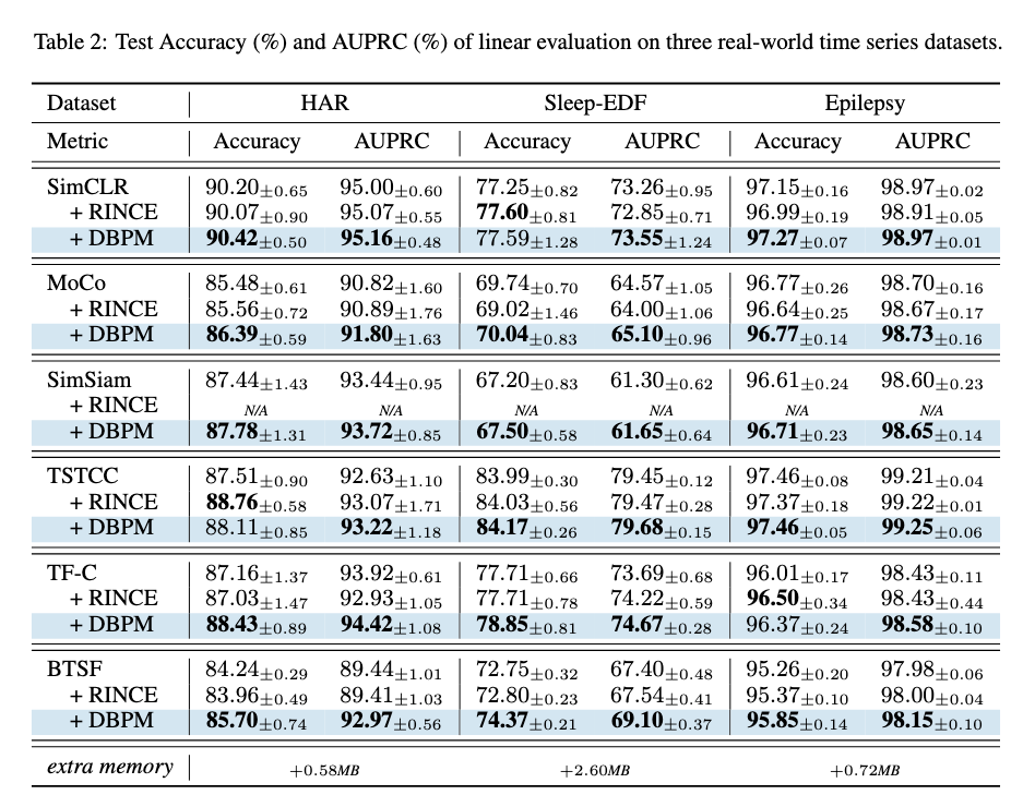
Experiments

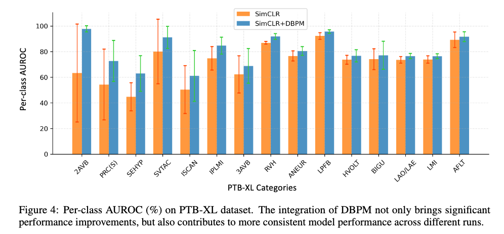
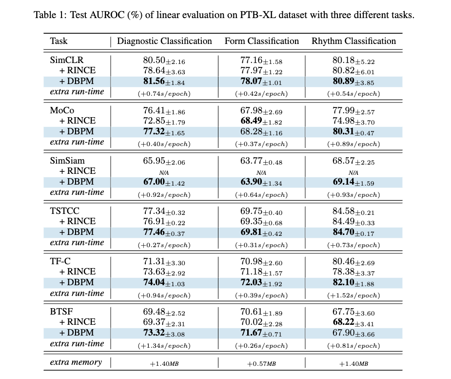
• RINCE: contrastive loss가 큰 애들만 패널티를 줌. 논문의 가정에 따르면 faulty positive pair에만 penalty가 가해진다고 볼 수 있음.

Conclusion

• In this paper, we investigated the bad positive pair problem in time series contrastive learning.
• We theoretically and empirically analyzed how noisy positive pairs and faulty positive pairs impair the quality of time series representation learned from contrastive learning.
• We further proposed a Dynamic Bad Pair Mining algorithm (DBPM) to address this problem and verified its effectiveness in four real-world datasets.